Wealthfront Automated Bond Portfolio Methodology White Paper

Introduction

Our Automated Bond Portfolios are designed for your short- to medium-term goals, assuming you are willing to accept a small amount of risk to potentially earn a higher yield than a savings account or Certificate of Deposit. We seek to provide a higher yield than our Cash Account, which is designed to hold cash short-term until you are ready to invest in the market. We construct the portfolio to have an expected annualized volatility, which is an estimate of dispersion of annual portfolio returns, of approximately 3%. This is roughly half of the expected volatility for the lowest risk versions of our Classic and Socially Responsible Automated Investing Account portfolios, which are designed for long-term investment and wealth accumulation. This white paper will discuss the methodology we use to construct our Automated Bond Portfolios. Our approach is designed to provide an attractive tradeoff between risk and after-tax, after-fee yield by investing in diversified and low-cost bond exchange-traded funds (ETFs). We ask tailored questions prior to opening an account to understand your specific tax situation and present an allocation based on this situation. We seek to maximize your after-tax yield with this personalized allocation and by applying tax-loss harvesting.

Introduction to Bonds

Bonds are debt securities issued by governments, agencies, or corporations. When an investor buys a bond, they are essentially lending money to the issuer for a fixed period of time. In return, the issuer promises to repay the value of the loan (referred to as the principal) at the end of the period (when the bond matures), plus, in most cases, interest payments (also called coupon payments) along the way. The size of the annual interest payments relative to the bond’s price is called the yield. In addition to yield, a bond may also experience price changes, measured in the form of price returns, which is the percentage change relative to its previous price. The sum of the two components gives us the total return of the bond.

Bonds compensate investors for taking on two types of risk:

1. Interest rate risk: This is the risk that the price of a bond will change due to interest rate changes. Assuming the issuer will make all coupon and principal payments as promised, the value of a bond is the sum of the present values of all its future payments. The present value for each payment can be calculated by discounting the payment back to the present day using the current interest rate corresponding to the amount of time until that payment occurs.

If interest rates rise, the present values of future payments, and thus the value of bonds, decrease. If interest rates decrease, the value of the bonds would increase.

To quantify interest rate risk, the overall sensitivity of a bond price to interest rates changes can be measured using a quantity called duration. Higher duration means higher interest rate risk. All else equal, the present value of a principal or interest payment will be more sensitive to a change in interest rates when time until the payment occurs is longer. This means that bonds with payments that are further in the future will be more sensitive to changes in interest rates (since the value of a bond is just the sum of the present values of all of its future payments). Expressed in years, the duration of a bond is the dollar-weighted average time to its payments. As an example, let’s imagine a bond pays $3 in one year, $3 in two years, and then $103 in three years. The final payment includes the principal, while the first two only include interest. The duration of this bond is:

Duration provides a single number measuring the sensitivity of a bond to interest rates. If interest rates rise (fall) by 1%, you can expect the value of a bond to decrease (increase) by 1% multiplied by the bond’s duration.

2. Credit risk: This is the risk of the issuer failing to pay the interest or principal back. When we discussed interest rate risk above, we made the assumption that the bond issuer made all of the bond’s payments as promised. This isn’t always the case—in some situations, the bond issuer may not have enough money and may stop making bond payments. This is known as defaulting on the bond. In general, bonds whose issuers are judged to have a higher chance of default will pay a higher rate of interest.

Credit rating agencies such as S&P, Fitch, and Moody’s evaluate the default risk of bonds and assign letter ratings based on their risk assessment. The bonds with the lowest level of default risk are rated AAA (or Aaa from Moody’s), while the riskiest (including bonds that have already defaulted) are assigned labels starting with C or D. Highly rated (BBB or better by S&P and Fitch, and Baa or better by Moody’s) bonds are called investment grade (IG), while riskier bonds are known as high yield (HY), or more colloquially junk bonds.

You can think of the rate of interest paid by a bond as the sum of three components:

1. The short-term “risk-free” rate—for example the rate paid by one-month US Treasury bills.
2. A duration premium—extra interest to compensate for lending for longer periods and taking on more interest rate risk. 
3. A credit premium—extra interest to compensate for the chance that the issuer might default.

Bonds are typically less risky than stocks for a few reasons. One reason for this is that almost all investment grade and majority of high yield bonds historically paid interest and returned principal on time according to the terms of the bonds. Another reason is that bondholders also have a more senior claim to a company's assets: In the event of company bankruptcy, bondholders would be paid first and stockholders would be paid afterwards if there were assets left. Thus, bondholders are more likely to recover their principal in adverse events.

Defining Bond Asset Classes and Sub-Asset Classes

We aim to build Automated Bond Portfolios that seek to maximize after-tax after-fee yield with a limited amount of risk using low-cost bond ETFs. The estimated volatility of the Automated Bond Portfolio is designed to be approximately halfway between our Cash Account, which has almost zero market risk, and the lowest risk versions of our Classic and Socially Responsible Automated Investing Accounts.

We start by defining a broad set of fixed-income asset classes and sub-asset classes as the universe of potential investments for our portfolios. These asset classes provide exposure to interest rate risk (duration) and credit risk in varying amounts, providing diversified sources of yield.

First, we have three treasury asset classes. Treasuries are issued by the US federal government and have minimal risk of default. Their interest payments are exempt from state income tax, thus providing tax-efficient income for investors in high-tax states.

Short-term Treasuries include Treasuries with remaining maturity less than approximately three years. We further divide this asset class into two subclasses:

• Ultra-short Treasuries with remaining maturity less than a year, and
• Short Treasuries with remaining maturity between one and three years

In addition to minimal default risk, short-term Treasuries also have low sensitivity to interest rate changes thanks to their short remaining maturities. They can provide steady, but often small, income streams. Because these bonds have low duration and essentially no default risk, their yields are usually low as well.

Medium-term Treasuries are Treasuries with remaining maturities between approximately three and 10 years. Medium-term Treasuries typically provide steady and slightly larger income streams than short-term Treasuries, as they are more sensitive to interest rate changes and thus often need to offer higher yield to attract investors.

• Investment grade (IG) corporate bonds include bonds with high quality ratings—for example, BBB or better from S&P and Fitch, or Baa or better from Moody’s. These ratings are considered strong and imply a relatively low default risk.
• High-yield (HY) corporate bonds include bonds with ratings below investment grade—for example BB+ and below from S&P and Fitch, or Ba1 and below from Moody’s. Since the default risk is higher it could lead to a higher yield than investment grade bonds to help compensate for this risk.
• Fallen angels are bonds that have recently been downgraded from Investment Grade to High Yield. These companies typically have the highest ratings among high-yield bonds (BB+ from S&P and Fitch, or Ba1 from Moody’s). Some may eventually make their way back to investment grade, but some others may stay in high yield.

Compared to Treasuries, corporate bonds generally offer higher yields due to their higher risk of default, lower liquidity, and the potential to be prepaid by the borrower.

Municipal bonds are debt issued by US state and local governments. Unlike most other bonds, municipal bonds’ interest is typically exempt from federal income taxes. They provide individual investors in high tax brackets a tax-efficient way to obtain income, low historical volatility, and diversification.

Foreign market bonds are debt securities issued mainly by foreign corporations, governments and quasi-government organizations (private companies providing governmental services). Foreign market bonds represent a significant part of the world bond market and serve as diversification from US bonds. This category includes two subclasses:

• Foreign developed market bonds are bonds issued by the governments and corporations of developed countries such as Japan, Germany, or the United Kingdom.
• Emerging market bonds are bonds issued by governments of emerging markets such as Mexico, China, or Brazil. Emerging market bonds generally have higher risk than developed market bonds, but they also offer the potential for higher yields.

Selecting Investment Vehicles

We use low-cost, liquid bond ETFs to construct our Automated Bond Portfolios. Bond ETFs are funds that hold a basket of bonds and are traded like stocks throughout the day on an exchange. Bond ETFs often track market capitalization-weighted indices, representing a specific segment of the bond market. Compared to single bonds, bond ETFs have the following advantages:

1. Diversification: Bond ETFs typically hold hundreds or even thousands of bonds, meaning they offer more diversification than a single bond. The bonds held by a bond ETF often have varying durations, which helps to reduce interest rate risk through diversification, and various issuers, which can lower credit risk through diversification. 
2. Liquidity: Bond ETFs are more liquid than bonds. That’s because bond ETFs are traded on exchanges much like stocks. Bonds, on the other hand, are generally traded over the counter. This means trades occur in a decentralized market in which market participants trade directly without a central exchange or broker. In addition, many bonds trade very infrequently. Some may not trade for weeks or even months.
3. Lower minimum: Most bonds have to be purchased in increments of $1,000, whereas bond ETF share prices are generally much lower.
4. Better bond pricing: Institutional investors, such as bond ETF providers, generally receive better bond pricing than individual investors as they purchase in large quantities. This better pricing for underlying bonds is subsequently reflected in the ETF pricing.
5. Less maintenance: As most bond ETFs do not mature, investors are not required to frequently buy new bonds to replace those that have matured.

On the other hand, ETFs are subject to management fees and other administrative expenses, which are captured in the expense ratio - the total annual cost of owning an ETF, expressed as a fraction of the investment size. However, we believe that the benefits of investing in bond ETFs typically far outweigh the expense ratio.

We chose ETFs that track an index instead of those that are actively managed, because actively managed funds on average underperform the market according to research (Bogle, 2009; Malkiel, 2012; SPIVA 2024). Among index-based funds, we prefer ones with low tracking error in relation to their benchmark indices. We chose ETFs instead of mutual funds for their liquidity and lower cost.

Some people believe that owning single bonds are safer than bond ETFs because as long as you hold a bond to maturity and it does not default you usually get back your principal, even if interest rates rise. While it’s true that such investors get back their principal (assuming there is no default), there are two potential issues with this logic. First, the no-default assumption may not always hold, especially for corporate or emerging market bonds. ETFs can help you diversify your default risk. Second, rising interest rates are typically a result of rising inflation. Buying power (or purchasing power), which indicates the amount of goods you can buy with the same amount of money, decreases by the amount of inflation every year. With a rising rate of inflation, your bond’s buying power decreases regardless of being held to maturity or not, as the same future payments can only buy fewer goods even if you hold the bond to receive them. By holding on to the same bond, you also miss the opportunity of buying into newly issued bonds with higher yield due to higher interest rate, which can help you combat inflation. ETFs, on the other hand, will periodically rebalance and include newly issued bonds.

Based on the considerations above, we believe that bond ETFs are the appropriate instruments to use for our portfolios. Table 1 shows the primary ETFs we chose for each asset or sub-asset class.

Source: Charles Schwab, Vanguard, BlackRock, VanEck, State Street, Wealthfront. Expense ratios are as of May 2024 and can change.

In addition to the primary ETFs above, we also use alternate ETFs that are highly correlated with the primary ETFs to carry out Tax-Loss Harvesting for our Automated Bond Portfolios. This is a service we offer for Classic and Socially Responsible Automated Investing Account portfolios as well. We aim to produce tax savings by selling ETFs that have declined in value to realize capital losses, and then buying a similar highly correlated ETF to maintain the portfolio’s risk and return profile. The capital losses generated can be used to offset capital gains and, if there are more losses than gains, up to $3,000 of ordinary income each year, thus lowering the investor’s taxes. Because bond ETFs tend to have lower price volatility than stock ETFs, we expect they will generally have fewer opportunities to harvest losses than in our other Automated Investing Account portfolios. However, our service will look for opportunities daily and aim to take advantage of them when available.

Portfolio Construction

Once we have a diverse set of instruments, we use a similar Mean-Variance Optimization similar to the one we use to construct our Classic and Socially Responsible Automated Investing Account portfolios. The main difference is that for Automated Bond Portfolios, we focus on maximizing after-tax yield rather than after-tax long-term return, as most of the earnings from bond ETFs are in the form of dividends. Similar to our Classic and Socially Responsible Automated Investing Account portfolios, we constrain the portfolio’s estimated volatility and set certain bounds for individual assets weights: we require weights of individual assets to add up to one. We also implemented additional asset bounds for diversification purposes. The output of this optimization is a portfolio that seeks to maximize one’s after-tax yield for a 3% estimated annual volatility level. 

We conduct the following optimization:

maximize: 𝑦 ′⋅𝑤

subject to:  𝑤′⋅𝛴⋅𝑤 = 𝜎²

𝑤 ⩾ 𝟢      

𝑤′⋅𝟙 = 1

𝑤 ∈ 𝑊 

where:

• y denotes the after-tax yield of each sub-asset class
• 𝑤 denotes the sub-asset class weights, which are being optimized
• 𝛴 denotes the sub-asset class covariance matrix
• 𝟙 is a vector of ones
• 𝜎 is the target portfolio volatility, 𝜎 = 3%. The expression 𝑤′⋅𝛴⋅𝑤 gives the expected annualized variance of the portfolio. The square root of this value is the annual volatility.
• 𝑊 represents a set of portfolios defined by extra constraints on the weights. “𝑤 ∈ 𝑊” means that the portfolio 𝑤 must satisfy these constraints. The extra constraints include lower and upper bounds on the individual asset and sector weights.

Yield metric choices

Our goal is to maximize the after-tax yield of the portfolio. Because of this, it is important that we use a yield metric that is timely. Since the yields of bond ETFs are highly influenced by interest rates, we want to understand any changes to expected yield when interest rates change. 

With this in mind, we chose the 30-day SEC yield as our yield metric. This is a standard calculation required by the Securities and Exchange Commission (SEC) for all bond funds, intended to allow for a fair comparison between different funds. It is calculated by applying the following formula over the last 30 days:

The innermost part of this formula is simply calculating the net-of-fee interest earned by the bonds in the fund as a fraction of the fund’s total size (number of shares outstanding multiplied by the price of each share). The rest of the formula converts this value to an annual percentage. There are two common ways to annualize a one-month return value, 𝑟. One is to calculate the annual value as (1+r)^12-1. This method assumes compounding of the monthly return. The other is to calculate the annualized return as 12r, which doesn’t factor in compounding. The formula for SEC yield splits the difference, computing a six-month value with compounding and then doubling it to get an annual figure. 

The 30-day SEC yield has some distinct advantages over other commonly used yield metrics such as trailing dividend yield, which is the average dividend yield over a prior period, calculated based on dividend payments made by the fund. The first advantage is timeliness: in times where interest rates are changing, a yield calculation that looks back three or twelve months will be much less representative of future yields than one that only looks back 30 days. In addition, funds tend to pay dividends on a monthly basis, but the exact date of the month varies. This makes yield estimates calculated using trailing dividends subject to noise from the specific timing of their payments. For example, calculating the yields of two bond funds using trailing dividends over the same period could be misleading if the period misses a dividend from one of the two funds. SEC yield, on the other hand, looks at yield from the underlying bonds within funds and does not have this issue, providing a more consistent comparison of yields between funds.

Another advantage of 30-day SEC yield is that it adjusts to the current market conditions. SEC yield reflects the latest yield based on current prices of the underlying bonds. This means the SEC yield can differ from the trailing dividend of an ETF, because ETF distributions are based on the prices of bonds when they entered the ETF portfolios. This difference is especially pronounced when interest rates are changing. For example, assume a 10-year maturity 2% coupon bond was purchased at par ($100) by an ETF. The ETF will pay out a $2 dividend (per $100) from this bond as long as it is in the portfolio. Now imagine that after five years, due to rising interest rates, the bond price drops to $95. Over the next five years until maturity, the bond price will gradually converge to $100 (its par or face value), meaning that there is an expected price appreciation of $1 per year. The SEC yield captures both the expected price appreciation and the coupon payments, and would be around 3% ($2 in coupons plus $1 in price appreciation per year, divided by a share price of $95) for an investor purchasing the ETF at the time. However, the ETF will continue to pay $2 per year in dividends, a rate of just over 2% ($2 divided by $95). Thus, the SEC yield more accurately reflects the total expected yield of underlying bonds.

Table 2 shows a comparison between the 30-day SEC yield and 12-month trailing yield for the primary ETF of each bond class as of May 2024. Trailing 12-month dividend yield is calculated as the average of monthly dividend yields over the past 12 months. For each month, dividend yield is the difference between monthly total return and ETF price return.

Source: Goldman Sachs, Charles Schwab, Vanguard, BlackRock, VanEck, State Street, CRSP

As of May 2024

Across the asset classes, Treasuries have lower 30-day SEC yields due to their minimal default risk. Corporate bonds and emerging market bonds have higher 30-day SEC yields than Treasuries due to their higher risk. Foreign developed market bonds have the lowest SEC yield due to lower benchmark rates in foreign developed countries than in the US.

The 30-day SEC yield also reflects the current state of the yield curve (the interest rates paid by US Treasuries as a function of their time to maturity), while other measures like the 12-month trailing dividend yield do not. In Table 2, the trailing 12-month dividend yield suggests a more steeply inverted yield curve, meaning short-term Treasuries have a higher yield than medium- or long-term Treasuries, despite having lower duration. This phenomenon is mainly driven by rate hikes in the past two years and expectations that interest rates will fall in the long term. However, as the rate drops approached, the curve started to flatten in 2024. The SEC yield curve, which is only very slightly inverted, reflects this change. The 12-month dividend yields, due to the nature of their construction, will take more time to reflect this change. 

Covariance matrix

The covariance matrix, 𝛴, in the first optimization constraint is used to calculate the theoretical risk of the portfolio. To construct this matrix, we use the same factor model methodology as in our Classic and Socially Responsible Automated Investing Account portfolios. The factor model estimates each asset's total return volatility (total return includes both price return and dividend yield) through two components:

1. Its exposure to common investment risk factors such as equity markets and interest rates
2. Its own idiosyncratic volatility that is not captured by the common factors

This methodology creates more robust risk and correlation estimates that are less impacted by one-time historical events compared to a simple covariance matrix calculated directly from historical returns of the asset classes.

Once we estimate the covariance matrix, we can separate it into two components: volatility of each sub-asset class and the correlation between sub-asset classes. We estimate the total return volatility of ETFs representing the sub-asset classes to be as follows:

 Source: Wealthfront

From the volatility estimates for each sub-asset class above, we can see that Treasuries generally have lower risk than corporate bonds of the same term, due to Treasuries’ minimal default risk. The exception is long-term Treasuries, which have slightly higher volatility than long-term corporates. This is because the long-term Treasuries ETF (Vanguard Long-term Treasury Bond ETF) has a longer duration than the long-term Investment Grade corporate ETF (Vanguard Long-term Corporate Bond ETF), and thus carries higher interest rate risk. Among corporate bonds, high-yield bonds have higher volatility than investment grade bonds of similar term due to their higher default risk. Emerging market bonds also have relatively high volatility due to their higher default risk. Within the same type of bonds, longer-term bonds have higher volatility than shorter-term bonds due to higher sensitivity to interest rate changes. Floating rate bonds have relatively low volatility due to their very low sensitivity to interest rate changes and high credit quality. 

Next we show correlation between various sub-asset classes. Correlation is shown in percentages:

 Source: Wealthfront

Since all sub-asset classes here provide exposure to different types of bonds, it is not surprising that most of the correlations are positive. However, as you can see, some correlation numbers are negative. These negative correlations are mostly between high-yield bonds, Treasuries, and floating rate bonds, due to their different risk profiles. This means those three asset classes are good diversifiers to each other. Even in the case of sub-asset classes that are positively correlated, we observe that most positive correlation numbers are significantly less than 100%, which means they still provide the benefit of diversification.

Constraints

In order to make sure the Automated Bond Portfolio is well diversified, we impose maximum bounds at two levels: the sector level and the granular sub-asset class level. Sectors are defined as Treasuries, corporates, and high-yield and emerging market bonds. Sub-asset classes are covered in detail in the “Defining Bond Asset Classes and Sub-Asset Classes” section above. Each sub-asset class includes a primary ETF we selected in Table 1 and its alternative ETFs. In stressed markets, asset volatilities may temporarily rise above their long-term estimates. This phenomenon is more prominent for assets with higher volatility. Thus, we cap the weight of higher risk sectors and sub-asset classes in an attempt to lessen the effect of short-term, high-volatility periods, with the size of the cap decreasing with the riskiness of the segment.

At the sector level, we believe a diversified portfolio should not have a single sector with more than half of the portfolio allocation. We make an exception for short and ultra-short Treasuries, which have low interest rate risk and extremely low default risk. Thus, we do not impose a maximum weight on Treasuries. To ensure diversification, we set a maximum 50% allocation for corporate bonds and the sum of high-yield and emerging market bonds. 

For most individual sub-asset classes, we generally impose a maximum allocation of 30%. Other respected sources (including Swensen, 2005) recommend similar maximum asset class allocations. The exceptions are high-yield bonds and emerging market bonds due to their higher risk relative to others in our universe. For high-yield bonds and emerging market bonds, the maximum is 20% to better manage the overall portfolio risk level in stressed markets.

As mentioned in the introduction section, we constructed the Automated Bond Portfolio to have roughly half of the expected volatility of the lowest risk versions of our Classic Automated Investing Account portfolios. Specifically, we constrain the estimated annual volatility of the portfolio to 3%. To put this number into perspective, 3% volatility is lower than most of the sub-asset classes in Table 3, including medium-term Treasuries. The resulting Automated Bond ETF portfolios are designed to have lower expected volatility than the Bloomberg US Aggregate Bond Index, a market capitalization-weighted aggregate index for US investment grade bonds. 

Personalization with Tax Rates

Bond ETF dividends are usually taxed as ordinary income, meaning they are usually subject to federal tax rates of up to 37%. This makes it important to optimize the portfolio based on yield net of expected tax rates. Certain types of bonds have tax exemptions on their dividends, which carry through to the dividends paid by ETFs that invest in these bonds and to the holders of such ETFs. We consider these tax advantages when designing our Automated Bond Portfolios:

1. Dividends from US Treasury ETFs are typically exempt from state tax. 
2. Dividends from municipal bond ETFs are generally exempt from federal income tax. If the underlying municipal bonds in the ETF are exclusively from the state an investor resides in, their dividends are usually exempt from state tax in addition to federal tax exemption.

There are seven federal income tax brackets, ranging from 10% to 37%. State income tax can vary widely across states. Several states such as Florida, Washington, and Texas do not have a state income tax at all. Other states have maximum rates of 8% or higher, with California topping the list with rates up to 13.3%. As our portfolio optimization’s objective is to maximize after-tax yield of the portfolio, different tax brackets will impact the objective function and potentially result in different allocations. However, we find that the optimal portfolio allocations are insensitive to the exact choices of tax rates. In fact, our research demonstrates that three representative portfolios—each optimized for a specific combination of state and federal taxes—are sufficient to deliver an expected after-tax yield within 0.02% of the optimal yield for any combination of tax rates. Table 5 shows the assumed state and federal tax rates used in the three representative portfolios. The medium tax level portfolio’s 24% federal tax rate and 4% state tax rate is approximately the median tax rate of our clients. For the low tax level portfolio, we chose the median federal tax rate below 24%. There are three federal tax brackets below 24%: 10%, 12%, and 22%, so we chose the median which is 12%. For state tax, we chose 0% because there are a number of states with no state tax regardless of income level, and even though 0% is the lowest possible rate, we wanted to make sure we were able to represent those states. For the high tax level portfolio, we chose the highest federal tax bracket, 37%, and a relatively high state tax rate of 10% because we found that this assumed tax rate combination ensured this portfolio is sufficiently different from the medium tax level portfolio and covers the highest tax bracket cases.

Table 5: Assumed Tax Rate of Representative Portfolios

In order to find the most tax-efficient portfolio for each client, we first infer your marginal federal and state tax rate based on your responses to the following three requests: your tax filing status, annual household income, and state of residence. We use marginal tax brackets because dividend earnings from the Automated Bond Portfolio will be in addition to the annual income you already earn. We also assume a standard deduction from the annual income when inferring the tax brackets. We then calculate your expected after-tax yield for each of the three representative portfolios, and assign you to the portfolio that delivers the better expected yield. Table 6 shows the assigned portfolio for every possible combination of state (rounded to the nearest percent) and federal tax rates based on this methodology.

Table 6: Optimal Portfolio Based on Marginal Federal and State Tax Brackets

 Source: Wealthfront

Figure 1 shows the optimal weights of asset classes and sub-asset classes in the three representative portfolios with assumed tax rates in Table 5. The low tax level portfolio contains some short-term corporate bonds, which have no tax exemptions but higher yield than short-term Treasuries, which they partially replace. The high tax level portfolio has less weight in floating rate bonds, which have no tax exemptions, and more weight in short Treasuries, which are exempt from state tax.

Source: Wealthfront

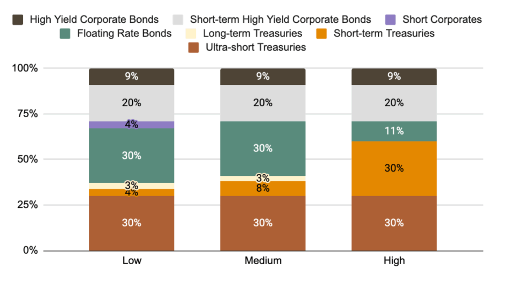
Perhaps surprisingly, neither portfolio includes municipal bonds. Although municipal bonds are typically exempt from federal taxes, their yields tend to be lower, and they are just as volatile as other bonds. As of May 2024, the yield on municipal bonds was low enough so that even with their tax advantages and relatively low correlation with other types of bonds, they didn’t earn any weight in the portfolios.

Table 7 compares the after-tax 30-day SEC yields of the primary ETFs for ultra-short Treasuries with municipal bonds for the three sets of representative tax rates. Yield and tax data are as of May 2024. For the low and medium tax levels, municipal bonds actually have lower after-tax yield than ultra-short Treasuries. For the high tax level, municipal bonds’ after-tax yield is 3.29% - 3.23% = 0.06% higher than ultra-short Treasuries, but since municipal bonds are much more volatile than ultra-short Treasuries (volatility of 6.5% compared to 0.2%), they are not nearly as attractive in a risk-adjusted sense.

Table 7: Pre and After-tax Yield

Source: Wealthfront, Goldman Sachs, Vanguard

As of May 2024, the low tax level portfolio had a pre-tax weighted-average 30-day SEC yield of 5.78%, while the medium tax level portfolio had a yield of 5.76% and high tax level portfolio had a yield of 5.62%, after deducting Wealthfront’s 0.25% annual advisory fee.

Table 8 shows each portfolio’s pre- and after-tax weighted-average 30-day SEC yield net of Wealthfront’s advisory fee as of May 2024. We also show the after-tax yield of the Wealthfront Cash Account for comparison. The Wealthfront Cash Account had a pre-tax annual yield of 5% as of May 2024.

Table 8: Portfolio Pre and After-tax SEC Yields Net of Advisory Fee

Source: Wealthfront

In terms of duration, we can see in Table 9 that all three portfolios have durations around 1.5 years as of May 2024. These durations are relatively low and indicate a low sensitivity to interest rate changes, resulting in less price volatility in changing rate environments.

Table 9: Portfolio Duration

Source: Wealthfront

Rebalancing and Ongoing Management

The composition of any portfolio will naturally drift as asset prices move. Even though the prices of bond ETFs are in general more stable than higher-risk asset classes (for example equities or real estate), it is still possible for certain sub-asset classes to outperform the others and alter the overall composition of a portfolio. 

A portfolio with composition different from the optimal allocation may result in:

1. Increased portfolio risk, if higher risk sub-asset classes grow beyond their recommended weight
2. Decreased after-tax yield, if lower after-tax yield sub-asset classes grow beyond their recommended weight

Therefore, we need to periodically rebalance the portfolio back to its optimal weight. We rebalance in a tax-optimized way that trades off deviation from the optimal portfolio with the tax consequences of selling appreciated assets. For Automated Bond Portfolios, rebalancing is less likely to cause capital gains because the portfolios pay regular dividends. This cash from dividends can be used to buy into assets whose weight becomes too small after the drift, thus reducing the need to sell existing holdings.

In addition to rebalancing, your optimal Automated Bond Portfolio may need to be adjusted over time. Over time, duration and credit premiums will vary, leading to different optimal portfolio weights. Wealthfront will periodically calculate new target weights for Automated Bond Portfolios using current yields and ask you if you would like to adopt the new targets. Any rebalancing needed with this adjustment will be carried out using the same tax-aware rebalancing that we use in all of our Automated Investing Account portfolios.

Furthermore, your investment goal and risk tolerance may change over time and these changes may impact which Wealthfront product(s) best fit those needs. Wealthfront recommends that you review your investment plan in detail every few years to make any necessary updates. We also remind you on a quarterly basis to keep us informed of any such changes.

Realized Results

This section discusses the realized performance of the Automated Bond Portfolio (ABP) strategies from March 30, 2023 (the inception date of the product) to December 31, 2023, focusing on total return earned by the portfolios as well as harvesting yield from our Tax-Loss Harvesting service.

Total Return

Table 10 shows the net of fee, pre-tax total return of the low tax and high tax  level Automated Bond Portfolio strategies. The medium tax level portfolio isn’t included because it wasn’t launched until late 2024. Total return includes both dividends received and price changes of the ETFs in the portfolios, and does not include any potential benefit from Tax-Loss-Harvesting. We calculate these values by first calculating the total return for every account with an account value of at least $5,000 enrolled in each tax variant of Automated Bond Portfolios for each trading day, and then compute a value-weighted average. We then compound daily returns over the full period.

The net of fee, pre-tax total return values of the two portfolios over this period are remarkably close, but this is due to chance. Over time we expect the pre-tax returns of the high-tax portfolio will be slightly lower than those of the low-tax portfolio, but only because each portfolio is optimized for after-tax return. For investors in high tax brackets, we expect the high-tax portfolio to outperform the low-tax portfolio after taxes.

Table 11 connects individual asset class performance to the overall portfolio. The table shows total (pre-tax) return of the primary ETF for each sub-asset class. Note that in the actual portfolios, we may use other ETFs highly correlated with primary ETFs to carry out tax-loss harvesting. Also, these allocations may vary over time. 

With the exception of long-term Treasuries, all bond asset classes within the Automated Bond Portfolio experienced positive returns over this period. The high-quality, short-duration assets (short and ultra-short Treasuries and floating-rate bonds) earned returns primarily from dividends, with price movement from changing expectations playing a much smaller role. The high-yield asset classes (high-yield and short-term high-yield corporate bonds) earned positive returns from both dividends and price appreciation. High-yield bonds, which have historically had higher correlations with equities than investment-grade bonds have had, rose in value along with equity markets as perceptions of default risk improved. Long-term Treasuries experienced small negative returns as price declines from rising expectations of long-term rates outweighed interest paid out as dividends. Figure 2 shows the breakdown of total returns into the dividend and price return components for each asset class.

Tax-Loss Harvesting

In this section, we examine the Tax-Loss-Harvesting results of the ABP strategies since their launch. For our analysis, we included client accounts enrolled in the Automated Bond Portfolio strategies with Tax-Loss Harvesting enabled and with account values of at least $5,000. We measure the performance of our Tax-Loss Harvesting service using harvesting yield, defined as the magnitude of losses harvested as a fraction of the portfolio value:

Harvesting Yield = Total Losses Harvested / Total Balance

Harvesting Yield is calculated daily and aggregated over the full period.

Since launch, both the low and high tax portfolios produced a harvesting yield in excess of 1.6%. The high tax portfolios harvested more losses due to their higher allocation to treasury asset classes, which had an overall drop in price.

Harvesting yield only measures the amount of losses harvested, not tax dollars saved. To estimate the true economic benefit, we need to multiply the harvested loss by an appropriate estimated tax rate. We apply estimated ordinary income tax rates to each account’s short-term harvested losses and estimated long-term capital gain rates to each account’s harvested long-term losses to calculate economic benefit from the tax loss strategy. Tax rates are combined marginal federal and state tax rates estimated using your self-reported income, state of residence, and marital status. We aggregate the economic benefit the same way as we do with harvesting yield, first across accounts for each day as a fraction of the total balance and then across days in 2023. The tax benefit as a fraction of total balance was 0.43% for low tax portfolios and 0.70% for high tax portfolios.

Conclusion

Wealthfront constructs Automated Bond Portfolios to address your need for an intermediate term investment product that is designed to provide a higher yield than our Cash Account while maintaining a lower risk than our Classic and Socially Responsible Automated Investing Account portfolios. Our Automated Bond Portfolios are designed to maximize after-tax, after-fee yield in a way that is optimized to your marginal tax rate. And finally we offer additional value through periodic portfolio rebalancing and tax-loss harvesting.

Bibliography

• Bogle, J. (2009). Common Sense on Mutual Funds. Wiley.
• Malkiel, B. (2012). A Random Walk Down Wall Street. W. W. Norton & Company.
• S&P Indices Versus Active (SPIVA) (2022), SPIVA Around the World
• Swensen, D. (2005). Unconventional Success. Free Press.

Disclosures

This Wealthfront Investment Methodology White Paper has been prepared by Wealthfront Advisers LLC (“Wealthfront”) solely for informational purposes only.  Nothing contained herein should be construed as (i) an offer to sell or solicitation of an offer to buy any security or (ii) any advice or recommendation to purchase any securities or other financial instruments and may not be construed as such. The information set forth herein has been obtained or derived from sources believed by Wealthfront to be reliable but it is not necessarily all-inclusive and is not guaranteed as to its accuracy and is not to be regarded as a representation or warranty, express or implied, as to the information’s accuracy or completeness, nor should the attached information serve as the basis of any investment decision. The information set forth herein has been provided to you as secondary information and should not be the primary source for any investment or allocation decision. This document is subject to further review and revision.

The information contained in this communication is provided for general informational purposes only, and should not be construed as investment or tax advice. Nothing in this communication should be construed as a solicitation or offer, or recommendation, to buy or sell any security. Any links provided to other server sites are offered as a matter of convenience and are not intended to imply that Wealthfront Advisers or its affiliates endorses, sponsors, promotes and/or is affiliated with the owners of or participants in those sites, or endorses any information contained on those sites, unless expressly stated otherwise.

Wealthfront Advisers and its affiliates do not provide legal or tax advice and do not assume any liability for the tax consequences of any client transaction. Clients should consult with their personal tax advisors regarding the tax consequences of investing with Wealthfront Advisers and engaging in these tax strategies, based on their particular circumstances. Clients and their personal tax advisors are responsible for how the transactions conducted in an account are reported to the IRS or any other taxing authority on the investor’s personal tax returns. Wealthfront Advisers assumes no responsibility for the tax consequences to any investor of any transaction.

The effectiveness of the tax-loss harvesting strategy to reduce the tax liability of the client will depend on the client’s entire tax and investment profile, including purchases and dispositions in a client’s (or client’s spouse’s) accounts outside of Wealthfront Advisers and type of investments (e.g., taxable or nontaxable) or holding period (e.g., short- term or long-term).

Wealthfront Advisers’ investment strategies, including portfolio rebalancing and tax loss harvesting, can lead to high levels of trading. High levels of trading could result in (a) bid-ask spread expense; (b) trade executions that may occur at prices beyond the bid ask spread (if quantity demanded exceeds quantity available at the bid or ask); (c) trading that may adversely move prices, such that subsequent transactions occur at worse prices; (d) trading that may disqualify some dividends from qualified dividend treatment; (e) unfulfilled orders or portfolio drift, in the event that markets are disorderly or trading halts altogether; and (f) unforeseen trading errors. The performance of the new securities purchased through the tax-loss harvesting service may be better or worse than the performance of the securities that are sold for tax-loss harvesting purposes.

Tax loss harvesting may generate a higher number of trades due to attempts to capture losses. There is a chance that trading attributed to tax loss harvesting may create capital gains and wash sales and could be subject to higher transaction costs and market impacts. In addition, tax loss harvesting strategies may produce losses, which may not be offset by sufficient gains in the account and may be limited to a $3,000 deduction against income. The utilization of losses harvested through the strategy will depend upon the recognition of capital gains in the same or a future tax period, and in addition may be subject to limitations under applicable tax laws, e.g., if there are insufficient realized gains in the tax period, the use of harvested losses may be limited to a $3,000 deduction against income and distributions. Losses harvested through the strategy that are not utilized in the tax period when recognized (e.g., because of insufficient capital gains and/or significant capital loss carryforwards), generally may be carried forward to offset future capital gains, if any.

The information in this document may contain projections or other forward-looking statements regarding future events, targets, forecasts or expectations that are based on Wealthfront’s current views and assumptions and involve known and unknown risks and uncertainties that could cause actual results, performance or events to differ materially from those expressed or implied in such statements. Neither the author nor Wealthfront or its affiliates assumes any duty to, nor undertakes to update forward looking statements.  Actual results, performance or events may differ materially from those in such statements due to, without limitation, (1) general economic conditions, (2) performance of financial markets, (3) changes in laws and regulations and (4) changes in the policies of governments and/or regulatory authorities. Any opinions expressed herein reflect our judgment as of the date hereof and neither the author nor Wealthfront undertakes to advise you of any changes in the views expressed herein.

Hypothetical expected returns information have many inherent limitations, some of which, but not all, are described herein. No representation is being made that any client account will or is likely to achieve performance returns or losses similar to those shown herein. In fact, there are frequently sharp differences between hypothetical expected returns and the actual returns subsequently realized by any particular trading program. One of the limitations of hypothetical expected returns is that they are generally prepared with the benefit of hindsight. In addition, hypothetical trading does not involve financial risk, and no hypothetical trading record can completely account for the impact of financial risk in actual trading. For example, the ability to withstand losses or adhere to a particular trading program in spite of trading losses are material points which can adversely affect actual trading results.  The hypothetical expected returns contained herein represent the application of the rule-based models as currently in effect on the date first written above and there can be no assurance that the models will remain the same in the future or that an application of the current models in the future will produce similar results because the relevant market and economic conditions that prevailed during the hypothetical performance period will not necessarily recur. There are numerous other factors related to the markets in general or to the implementation of any specific trading program which cannot be fully accounted for in the preparation of hypothetical performance results, all of which can adversely affect actual trading results. Hypothetical expected returns are presented for illustrative purposes only. No representation or warranty is made as to the reasonableness of the assumptions made or that all assumptions used in achieving the returns have been stated or fully considered. Changes in the assumptions may have a material impact on the hypothetical returns presented.

Past performance is no guarantee of future results, and any hypothetical returns, expected returns, or probability projections may not reflect actual future performance. Actual investors may experience different results from the expected or hypothetical returns shown. There is a potential for loss that is not reflected in the hypothetical information portrayed. The expected returns shown do not represent the results of actual trading using client assets but were achieved by means of the retroactive application of a model designed with the benefit of hindsight.

No representation or warranty, express or implied, is made or given by or on behalf of the author, Wealthfront or its affiliates as to the accuracy and completeness or fairness of the information contained in this document, and no responsibility or liability is accepted for any such information.  By accepting this document in its entirety, the recipient acknowledges its understanding and acceptance of the foregoing statement.

Investing in bond ETFs involves risks, including tracking error, credit risk, interest rate risk, liquidity risk, and the possibility of incurring capital gains taxes during the fund's rebalancing. Unlike individual bonds, bond ETFs do not provide a fixed maturity date or guarantee of principal repayment at maturity. Investors should carefully consider these risks before making investment decisions. Past performance is not indicative of future results.

The Annual Percentage Yield (APY) for the Cash Account may change at any time, before or after the Cash Account is opened. The APY for the Wealthfront Cash Account represents the weighted average of the APY on the aggregate deposit balances of all clients at the program banks. Deposit balances are not allocated equally among the participating program banks.

Cash Account is offered by Wealthfront Brokerage LLC (“Wealthfront Brokerage”), a Member of FINRA/SIPC. Neither Wealthfront Brokerage nor any of its affiliates are a bank, and Cash Account is not a checking or savings account. We convey funds to partner banks who accept and maintain deposits, provide the interest rate, and provide FDIC insurance. Investment management and advisory services--which are not FDIC insured--are provided by Wealthfront Advisers LLC (“Wealthfront Advisers”), an SEC-registered investment adviser, and financial planning tools are provided by Wealthfront Software LLC (“Wealthfront”).

All investing involves risk, including the possible loss of money you invest, and past performance does not guarantee future performance. Historical returns, expected returns, and probability projections are provided for informational and illustrative purposes, and may not reflect actual future performance. Please see our Full Disclosure for important details.

Wealthfront Advisers, Wealthfront Brokerage and Wealthfront are wholly owned subsidiaries of Wealthfront Corporation.

Copyright 2024 Wealthfront Corporation. All rights reserved.

⇧ Back to top