Risk Parity Whitepaper
Introduction
While the allocations of traditional portfolios appear “balanced,” often a large share of their overall risk results from their allocation to equities, which are considerably riskier than other asset classes. As a result, investors seeking to achieve high expected returns by increasing their allocation to equities are commonly forced to hold portfolios that are highly concentrated from a risk perspective.
Risk parity is a portfolio diversification strategy which addresses risk concentration by first equalizing the risk contributions of each asset class, and then uses leverage to scale the risk of the resultant allocation to the desired volatility. The academic research, which inspired the strategy, dates back to the 1970s and the strategy itself has been employed by institutional and high-net worth clients since the 1990s.
This whitepaper explains how one would create a risk parity portfolio and examines the hypothetical backtested performance of this time-tested, rules-based approach to portfolio construction.
Methodology
We construct a hypothetical risk parity strategy in two steps. First, we create an unlevered portfolio that balances the risk contributions of the constituent asset classes. Relative to traditional portfolio construction methods, such as mean-variance optimization, the resulting portfolio will generally overweight low risk asset classes (bonds) relative to high risk asset classes (equities). As a consequence, it will tend to have a relatively low volatility.
Second, we apply leverage to achieve a target level of volatility. In practice, this can be achieved through explicit borrowing or the use of derivatives like a total return swap. The volatility of the unlevered risk parity portfolio will generally change over time due to changes in the volatility of the underlying asset classes. By periodically adjusting the amount of leverage, the strategy is able to target a constant level of volatility, in contrast to traditional portfolios whose volatility changes dramatically over time.
Balancing Risk Contributions
The essence of a risk parity strategy is to equalize the risk contributions of each asset class in the portfolio. In order to mathematically define these risk contributions, one first needs to settle on a measure of portfolio risk. While there are many possible choices, a commonly chosen metric for constructing risk parity strategies is the portfolio’s volatility (i.e. the square root of the portfolio’s variance). The virtue of using volatility is that it allows for an elegant additive decomposition of the portfolio’s volatility into contributions from the underlying asset classes.
If we let ω denote the portfolio weight vector, and Σ denote the variance-covariance matrix of asset returns, the portfolio volatility — written as a function of the weights — is expressed by:

where the prime denotes the matrix transpose. The risk contribution of each asset class is then obtained by multiplying elementwise the portfolio weights with the partial derivative of the portfolio’s volatility. The elementwise multiplication is denoted by ⊙ in the definition below.

The risk contributions of all the asset classes sum to the portfolio’s volatility. Equivalently, if the risk contributions are scaled by the volatility they will sum to one. When searching for the portfolio weights that equalize the risk contributions, we additionally impose the constraints that: (a) the weights are strictly positive (i.e. we do not allow for shorting) and (b) the sum of the weights has to equal one (i.e. the portfolio is unlevered).
A striking feature of this portfolio construction methodology is that it requires an estimate of the variance-covariance matrix of asset returns, Σ. This is distinct from traditional portfolio construction methods, such as mean-variance optimization, which require estimates of both the expected returns (“means”) and risks (“variances”) for each of the asset classes. This represents a potentially meaningful benefit as asset class expected returns are considerably more difficult to estimate than variances (Merton (1980)).
To illustrate the computation of portfolio risk contributions, Table 1 examines a traditional 60/40 equity/bond portfolio, which is commonly regarded as a “balanced” allocation. For the purposes of illustration, let’s assume equities have an annualized volatility of 15%, bonds an annualized volatility of 5%, and the two assets have a correlation of -0.50. The table below displays the portfolio weights, volatilities, risk contributions (which sum to the portfolio volatility), and the risk contributions divided by the portfolio volatility (which sum to one).
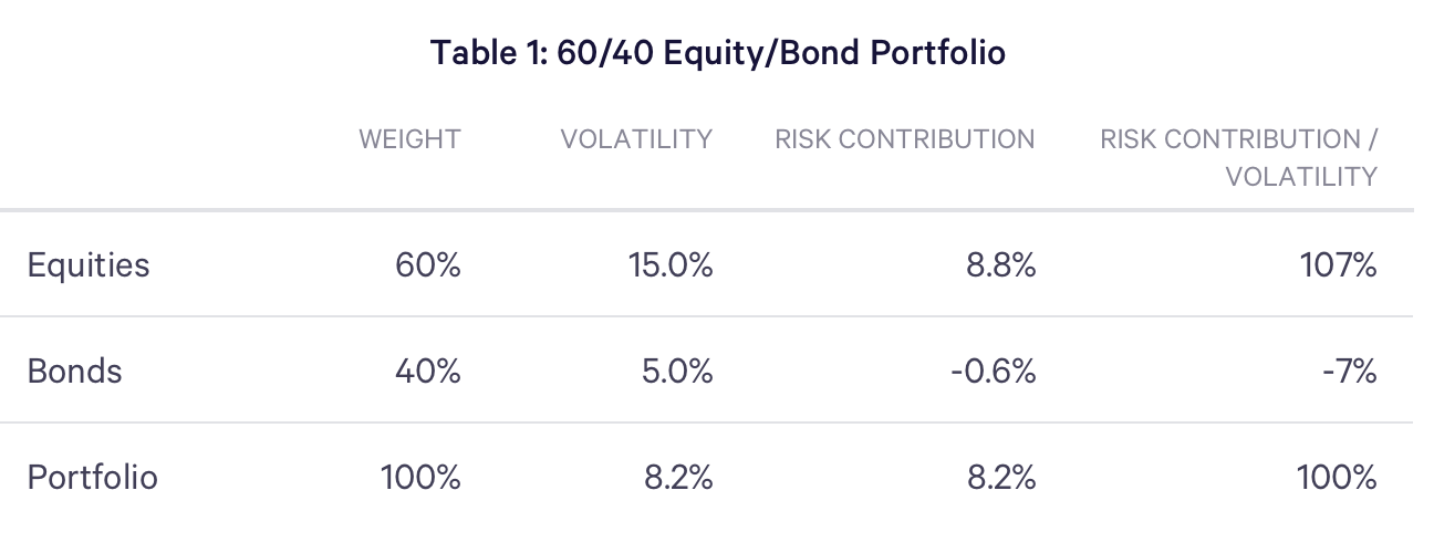
The computation of the relative risk contributions exposes that the risk of the supposedly “balanced” 60/40 portfolio is actually dominated by equities, so much so that their relative risk contribution even exceeds 100% (8.8% vs. 8.2% for the entire portfolio). Put differently, bonds are not only less risky than equities, they play an important role as a risk diversifier through their negative correlation with equities. To solve for an equity/bond portfolio where asset class risk contributions are equalized we use a numerical solver to obtain the results in Table 2.
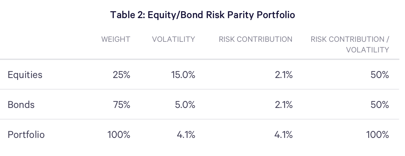
Relative to the traditional “balanced” portfolio, the risk parity portfolio increases the allocation to bonds and decreases the allocation to equities. As a result, the portfolio achieves a considerably lower volatility than the original 60/40 equity/bond allocation (4.1% vs. 8.2%). To obtain a comparable level of portfolio risk with the 60/40 portfolio, the investor would need to leverage the risk parity portfolio. The quantity of leverage necessary to achieve a given target volatility is equal to the ratio of the target volatility and the volatility of the unlevered portfolio:

In the above case, matching the volatility of the 60/40 equity/bond allocation would require leveraging the risk parity portfolio by a factor of 2x (8.2%/4.1%). In other words you would have to borrow an amount equal to the value of an unlevered portfolio.
Impact of Time-Varying Asset Class Risk
In practice, asset class volatilities (and correlations) can change meaningfully over time both in absolute terms (e.g. the volatility of equities spikes considerably during times of market declines) and relative to one another. To illustrate this, Figure 1 plots the realized annualized volatility for U.S. equities and U.S. bonds over the last two decades, using a rolling window of six months of daily returns.

Figure 1 illustrates three important phenomena. First, the volatility of individual asset classes varies over time, such that the composition of an equity/bond risk parity portfolio would also change over time. Importantly, the changes in asset class volatilities are somewhat persistent (i.e. periods of high volatility are followed by gradual declines), such that past levels of volatility can be used to forecast future levels of volatility for short horizons. This phenomenon was first observed by Robert Engle, Professor of Management and Financial Services at New York University, who developed a class of econometric models to measure and forecast the volatility of time series data. These models, known as autoregressive conditional heteroskedasticity models (or ARCH models), were subsequently recognized with the 2003 Nobel Prize in Economics. Applying such models to a moving window of daily historical data allows us to construct a forward-looking estimate of the variance-covariance matrix of asset returns, Σ, which can in turn be used to compute portfolio allocations that equalize the risk contributions of various asset classes.
To illustrate these effects, suppose we continue with our simplified stock/bond example, but additionally assume the market entered an extended downturn. In such periods, ARCH models typically forecast a higher level of volatility. For the sake of illustration, let’s assume the forecasts of equity and bond volatilities rise to 40% and 10%, well within the historically observed range of volatilities displayed in Figure 1. Based on these forecasts, the risk parity composition would change as displayed in Table 3, reallocating even further away from equities and toward bonds.
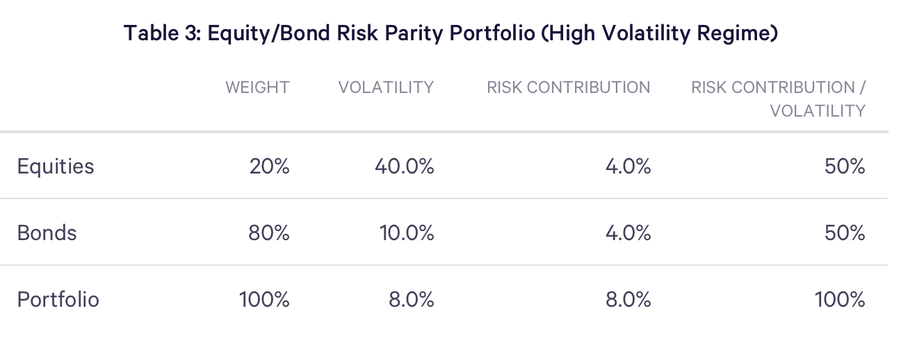
The shift in asset class volatilities (holding the correlations fixed) increases the risk of the overall portfolio from 4.1% in the baseline case (Table 2) to 8.0% (Table 3). For comparison, under the same volatility assumptions, the shift in the volatility of a portfolio rebalanced to a constant 60/40 equity/bond allocation would have been even more dramatic, reaching 22.3%, or nearly triple its baseline level (Table 1). This illustrates that portfolios targeting fixed portfolio weights can experience very significant variation in their risk over the business cycle, with volatility rising rapidly following large market declines (e.g. 2008 credit crisis).
Finally, at these increased volatilities, if the risk parity investor continued to target an annualized volatility of 8.2%, i.e. the annualized volatility of the 60/40 portfolio in its baseline case (Table 1), the required portfolio leverage would be 1.025x (8.2% from the original allocation/8.0% from the high volatility case). Thus the required portfolio leverage declines from a factor of 2x in the baseline scenario to roughly 1x in the stress scenario.
The above examples illustrate the key features of applying the risk parity portfolio construction methodology, while targeting a fixed level of portfolio risk:
-
- The allocation of a portfolio equalizing risk contributions changes over time based on the forecasts of volatilities and correlations among the asset classes.
-
- The quantity of leverage required to achieve a fixed level of portfolio volatility varies over time.
Accessing Leverage
As the above examples illustrate, equalizing the risk contributions of the asset classes, and achieving a fixed level of portfolio volatility are distinct tasks. The first task can be achieved by applying the portfolio construction methodology described above to one’s forecast of the variance-covariance matrix of asset class returns. The second task requires applying a time-varying quantity of leverage.
The simple way to apply leverage is to directly borrow money. Unfortunately it is very difficult to find a lender who will offer financing at a reasonable rate if the portfolio grows to be very large. An alternative and more practical way to generate leverage is to enter into a “Total Return Swap” with a counterparty like a trading desk at a large bank.
In a total return swap, one party (the portfolio manager) agrees to make interest payments based on a set rate in return for the other party (the bank) committing to make payments based on the total return of an underlying asset. The set rate is commonly expressed as a combination of a reference rate, such as OBFR (the Overnight Bank Funding Rate), and a spread. The precise details of such a transaction would be governed by an International Swaps and Derivatives Association (ISDA) agreement negotiated between the two parties.
In the case of using a total return swap to build a risk parity portfolio, the portfolio manager might agree to pay an interest rate of OBFR plus 50 basis points in return for the bank trading desk committing to deliver the return from the index funds that represent the risk parity portfolio of the sort found in Tables 2 and 3. Banks have very sizable balance sheets that enable them to offer very large total return swaps. They generate a profit based on the spread they charge over OBFR because they can borrow for less than OBFR. The total return swap makes sense to the portfolio manager as long as the return of the index funds acquired in the levered risk parity portfolio minus the rate charged by the bank is superior to that of other risk-matched investments.
Let us illustrate with an example. Suppose the portfolio manager and the bank enter into a one month swap with a notional amount of $100 million and a financing rate of 1%. If the underlying risk parity portfolio appreciated by 2.5% over one month, the bank would send the portfolio manager an amount equal to $2.5 million (2.5% * $100 million) at the end of the month, and the portfolio manager would send the bank a payment of $83,333 (1.0% * $100 million * 1/12). In practice, the parties commonly only exchange the net payment, so here the portfolio manager would actually receive a payment of $2,416,667. If the underlying asset depreciated by 2.5% over one month, the bank would have no payments to make, while portfolio manager would have to send an amount equal to the depreciation plus the interest payment ($83,333), for a total payment of $2,583,333 ($2.5 million + $83,333). More generally, the profit-and-loss, or PnL, of the swap can be written as:
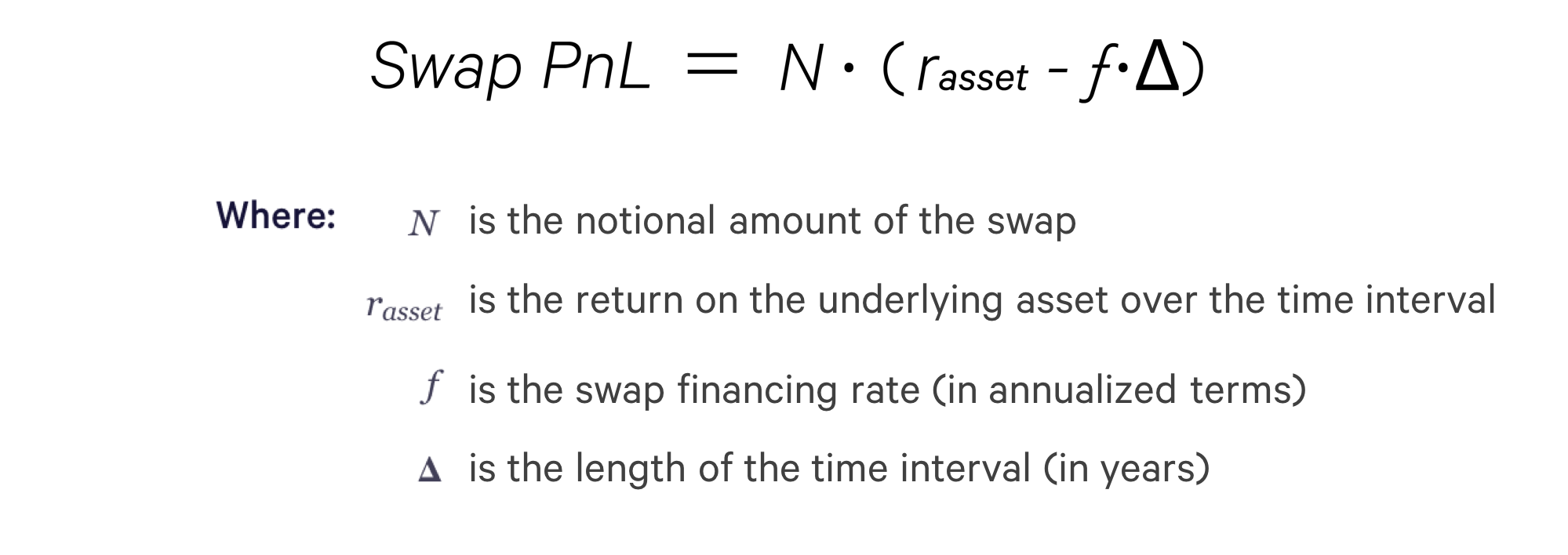
Notice that the payoff of the swap is economically equivalent to the portfolio manager having purchased an amount of the underlying asset equal to the swap’s notional value, N, while borrowing the funds at a rate determined by the set financing rate, f, equal to (OBFR + spread). In this sense, a total return swap provides the portfolio manager synthetic leveraged exposure to the underlying asset.
In order to guard against the risk that the portfolio manager is unable to make the promised payment in the event that the underlying asset depreciates significantly (i.e. counterparty risk), the bank will generally demand the posting of collateral at the inception of the transaction. This collateral amount may be further adjusted over the course of the life of the swap based on daily changes in the value of the underlying asset. Typically, the bank would accept the posting of cash or U.S. Treasury securities as collateral with the precise type and quantity determined by the ISDA agreement.
To clarify the amount of leverage implicit in a total return swap arrangement, suppose the portfolio manager actually had only $50 million in assets, but wanted to obtain exposure to $100 million of the underlying asset. It could either do this by buying $100 million of the underlying asset using $50 million of its own funds and borrowing the other $50 million, or it could enter into a total return swap with a notional of $100 million, while posting the $50 million as collateral for the swap. In both cases, the leverage — measured as total asset exposure divided by the investor’s capital in the transaction — in this transaction is equal to 2x.
From here, one can see that by entering into a total return swap where the “underlying asset” is defined to be a multi-asset class portfolio with equalized risk contributions, one is in position to periodically adjust both the composition of the reference portfolio, as well as, the quantity of leverage applied. These features make total return swaps an efficient mechanism for the implementation of a risk parity strategy.
Risk Parity Strategy Backtest
This section explores the historical performance of a hypothetical risk parity strategy from June 1, 1996 to September 30, 2017, which represents the period for which we have realized return data for commercially available funds envisioned to comprise the hypothetical portfolio.
The key assumptions of the backtest are as follows:
-
- Asset Classes: The risk parity portfolio is constructed from index funds that represent a combination of seven asset classes, which includes US Equities, Foreign Developed Equities, Emerging Market Equities, US Bonds, Emerging Market Bonds, Energy Stocks, and REITs.
- Reference Portfolio: The returns of each asset class are based on the returns of broadly diversified index exchange traded funds or mutual funds, and are computed net of the management fee of the respective fund. We rely on data for mutual funds only when comparable data for the exchange traded fund is unavailable.
- Fees and Trading Costs: The returns on the reference portfolio are computed net of management fees charged by the underlying funds. However, the strategy backtest does not incorporate costs associated with trading the funds. Also, unless stated otherwise, the strategy returns are presented before the deduction of a management fee.
- Rebalancing: The risk parity portfolio is rebalanced monthly.
- Volatility Target: The strategy targets a constant annualized volatility of 12%.
- Leverage: The strategy is assumed to have been able to obtain leverage using a total return swap with the unlevered risk parity portfolio as the underlying asset at a financing rate equal to the 1-month Treasury Bill rate plus a spread of 75 basis points. Swap payments are assumed to be exchanged at each month-end. The strategy leverage is capped at a maximum of 3x. The assumed financing rate is hypothetical, and currently higher than what we have been offered; a higher (lower) financing rate reduces (increases) the reported backtested returns.
- Collateral: The assets of the hypothetical strategy are assumed to be fully invested in 1 Month Treasury Bills, which are available for use as collateral to establish and maintain the total return swap position.
Portfolio Construction
At each month-end we construct a forecast of the one-month asset class variance-covariance matrix using a rolling, backward-looking window of daily returns. Using this estimator, Σ, we compute the composition of the unlevered risk parity portfolio, ω, as described in the first section of this white paper. Figure 2 displays the variation in the composition of the unlevered portfolio over time. The allocations to US bonds and emerging market bonds dominate the composition of the portfolio. Specifically, over this time period the average allocations to the seven asset classes were: US Equities (7%), Foreign Developed Equities (7%), Emerging Market Equities (6%), US Bonds (52%), Emerging Market Bonds (14%), Energy Stocks (6%), and REITs (8%).
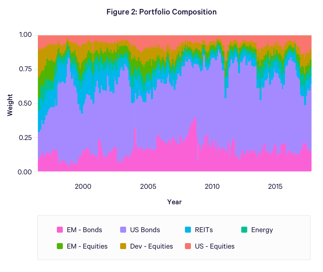
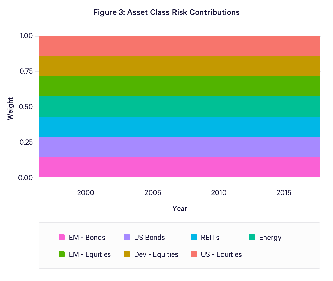
The combined allocation to the two bond asset classes was particularly large in the period following the Long Term Capital Management (LTCM) crisis (August 1998) and the credit crisis (Fall 2008). However, a key difference between these two events is that during the LTCM crisis emerging market bond volatilities spiked alongside equity volatilities, such that the portfolio tilted disproportionately toward safe US bonds, rather than emerging market bonds. During the second of these events, allocation to both types of bonds rose, since the reallocation was driven primarily by the disproportionate rise in the forecasts of equity market volatilities (US, Foreign Developed, and Emerging Market). Figure 3 illustrates how the risk parity strategy equalized the relative risk contribution of each asset class over time.
Portfolio Leverage
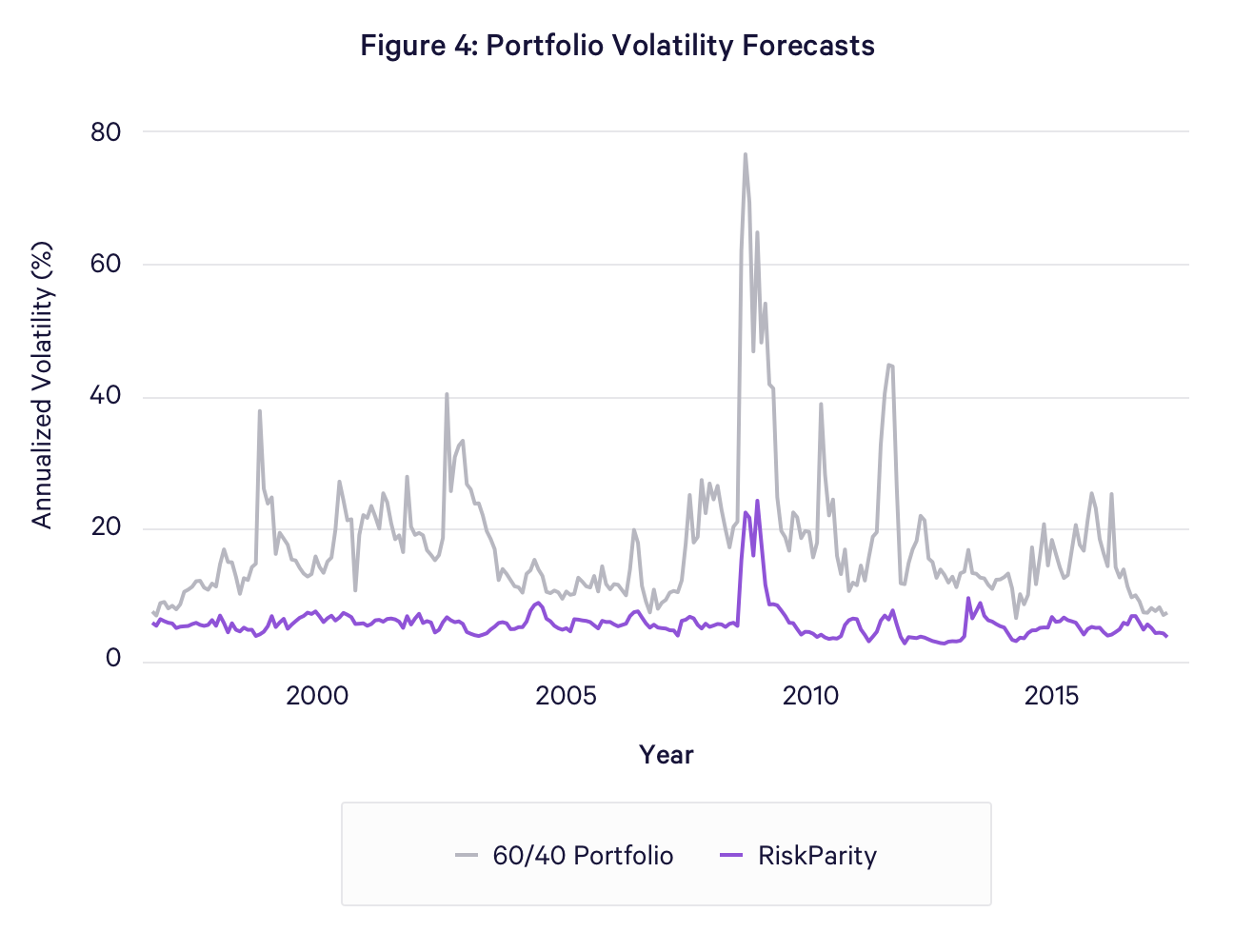
At each month-end we use the composition of the unlevered risk parity portfolio, ω, to compute the forecast of its volatility over the upcoming month as:
The time series of these forecasts, along with the corresponding forecasts for the 60/40 equity/bond portfolio is plotted in Figure 4. The chart indicates that the annualized volatility of the unlevered risk parity portfolio historically averaged 5.5%, with only a brief period around the fall of 2008, when it exceeded 20%. For comparison, the one-month ahead volatility forecast for the 60/40 equity/bond portfolio averaged 10.9%, but exhibited much greater variation, rising to over 75% at the height of the credit crisis in 2008.
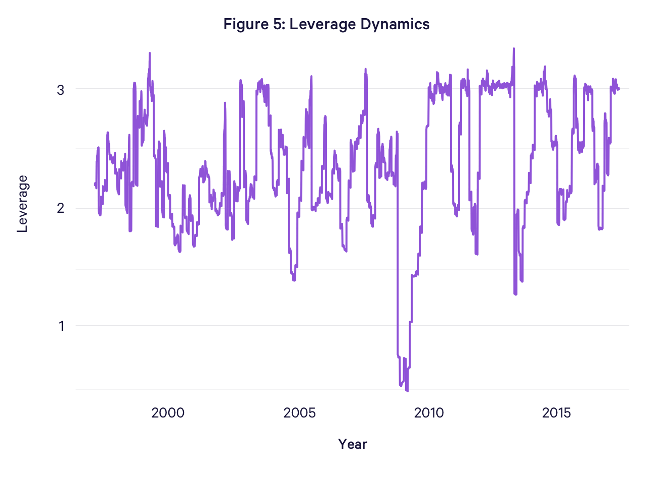
At each month end, the quantity of leverage that has to be applied to the risk parity portfolio in order to achieve the targeted annualized volatility is 12% / σ(ω). For example, when the forecasted volatility of the unlevered risk parity portfolio is 8%, the leverage is equal to 1.5. When the forecasted volatility exceeds 12%, the risk parity strategy effectively deleverages by mixing the target portfolio with Treasury bills. Finally, we cap the maximum leverage that the strategy is able to deploy at each month end to 3x, such that if the σ(ω) drops below 4%, the backtested strategy would be unable to reach its target volatility of 12%. As Figure 5 illustrates, this happened in a very small number of months. The leverage of the strategy is reset at each month end when the portfolio is rebalanced, and is otherwise allowed to vary freely within the month. As a result, if the portfolio experiences a gain within the month, the leverage will decline because the swap notional value remains unchanged. Conversely, if the portfolio experiences a loss within the month, the leverage will rise above the value at the reset date. Even though portfolio leverage is capped at 3x at the reset dates, it can increase beyond that amount intra-month. Figure 5 displays the time series of the daily leverage values over the full backtest period. We find that the average leverage necessary to achieve an annualized volatility target of 12% has been approximately 2.3, rising to a maximum value of 3.3 and a minimum value of 0.5.
Results
Having constructed the time series of the unlevered risk parity portfolios and determined the quantity of leverage necessary to achieve the desired target volatility, we can compute the hypothetical, backtested returns for the strategy. These are summarized in Table 4. The backtested strategy achieved an annualized return of 11.3% during the more than 20 year backtest. The annualized volatility of the realized returns equaled 13.3%, only slightly overshooting the targeted risk of 12%.
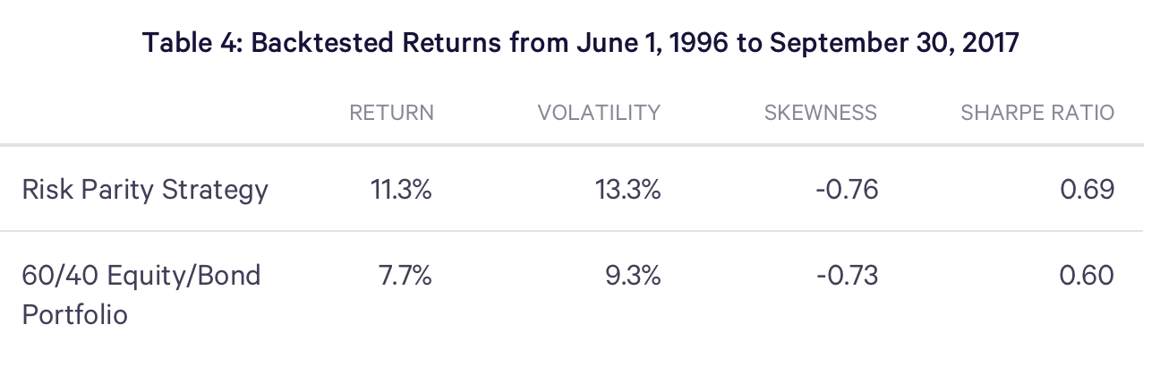
When compared to the traditional 60/40 portfolio, the risk parity strategy achieved a higher mean return, but did so with a higher level of volatility. To account for this, we computed the Sharpe Ratios of the two strategies, which indicates that the risk parity strategy delivered an 18% improvement in risk-adjusted return. This replicates a series of well-documented findings, dating back at least to Black, Jensen, and Scholes (1972), indicating that leveraging lower risk assets tends to deliver higher risk-adjusted returns than investing in a portfolio of riskier assets. One hypothesis advanced to account for this finding is that investors face limits to accessing leverage. Consequently, risk tolerant investors who desire a high risk portfolio, but cannot lever a relatively lower-risk portfolio, must overweight risky assets. This causes high risk assets to become overpriced relative to an equilibrium with unconstrained access to leverage. In turn, the expected returns on these assets are lower resulting in more modest risk-adjusted returns.
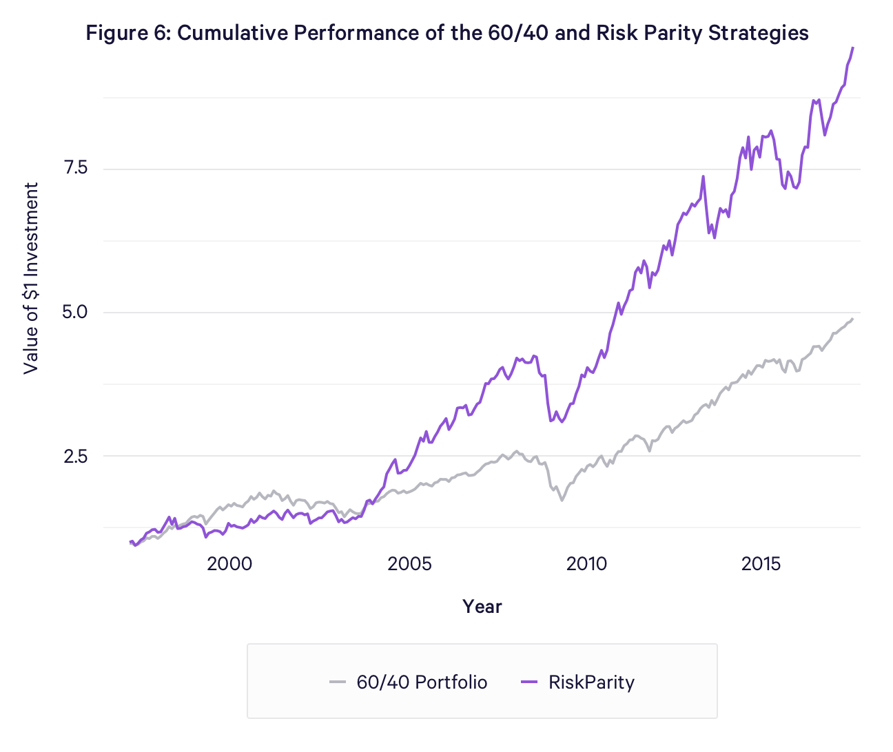
The cumulative returns of the two strategies are presented in Figure 6. With the exception of the early part of the sample (1996 – 2000), which coincides with the Internet Bubble, the risk parity strategy appreciates at a consistently higher rate than the 60/40 portfolio. The underperformance in the initial period reflects a comparatively low allocation of the risk parity strategy to equities during a time when they experienced unusually rapid appreciation.
Performance Comparisons
This section compares the backtested performance of the risk parity strategy with the performance of a diversified portfolio, as well as, with the realized, historical performance of two well-known risk parity funds.
Comparison with Diversified Portfolio
Table 5 compares the hypothetical backtested returns of the risk parity strategy with the backtested returns of a globally diversified portfolio, constructed using mean-variance optimization, that has a similar volatility as the risk parity strategy over the comparison period. The data are based on monthly returns from June 1, 1996 to September 30, 2017, matching the full length of the Risk Parity strategy backtest. All figures in the table are annualized.

Hypothetical performance results of the Risk Parity Strategy and the Diversified Portfolio are presented for illustrative purposes only, and do not represent performance returns of any actual strategies or accounts managed by Wealthfront or its affiliates for the periods shown. The Diversified Portfolio employs the allocation of the Wealthfront taxable portfolio with Risk Score 8.0. Please refer to the disclosure section below for a description of how the backtested returns of the Wealthfront Taxable Portfolio were determined.
The data suggests that an investor in a globally-diversified portfolio employing the same asset allocation as a taxable Wealthfront Risk Score 8.0 portfolio could have increased her pre-tax, net-of-fee expected return by allocating a portion of her portfolio to the risk parity strategy. Determining the optimal allocation to the strategy requires forming a forward-looking assessment of its returns, and determining how it covaries with the other investable asset classes. The analysis indicates that investors could increase their pre-tax, net-of-fee returns by up to 0.25% per year, even though allocations are restricted to be no larger than 20% of the portfolio. We apply this restriction to ensure clients can continue to benefit from Wealthfront’s other value-added investment features, such as Tax-Loss Harvesting and Portfolio Line of Credit.
Comparison with Existing Risk Parity Funds
Table 6 compares the hypothetical backtested returns for the risk parity strategy net of a 0.25% management fee payable monthly with the realized fund returns for Bridgewater Associates, and AQR Capital Management net of their respective fees. For Bridgewater, we compare performance with their 12% target volatility All Weather Fund; for AQR, we compare performance with a 60/40 blend of their low- and high-volatility risk parity mutual funds. The two funds have target volatilities of 10% (AQRIX) and 15% (QRHIX), respectively, such that the blend would have a target volatility of 12%, under the assumption of perfect correlation between the two funds. The comparison with Bridgewater is based on monthly returns from June 1, 1996 to September 30, 2017; the comparison with AQR is based on returns from December 1, 2012 to September 30, 2017. In both instances, these represent the longest time period over which a common set of data is available. All figures in the table are annualized.
 This information is for illustrative purposes only and does not represent the performance of any strategies or accounts managed by Wealthfront or its affiliates. The implementation of the investment strategies of the Bridgewater All Weather Fund, and AQR Risk Parity Fund may differ greatly from one another, and differ greatly from the assumptions made in deriving the backtested performance of the Risk Parity Strategy.
While the hypothetical backtested results compare favorably with the actual, realized returns achieved by the commercially available funds, investors should not expect the strategy to continue outperforming the commercial funds by a similar margin. To highlight the wide range of possible outcomes of the Risk Parity Strategy relative to the other funds, we report its Tracking Error. The Tracking Error measures the annualized standard deviation of the differences in monthly returns between a given fund and the Risk Parity Strategy. The large magnitudes of the Tracking Error reflect that the Risk Parity Strategy was designed to deliver the return from applying a simple, rules-based approach to portfolio construction, rather than to track the returns of either fund closely.
Moreover, any comparison of actual realized returns with backtested data must be taken with a significant grain (perhaps even a hill) of salt. Specifically, the backtest: (a) does not incorporate trading costs (commissions and bid-ask spreads); (b) assumes the counterparties of the total return swaps were willing to extend leverage at all points along the way; and, (c) assumes a fixed financing spread, which may not have been feasible historically.
Sensitivity to Interest Rates
Due to its large exposure to bonds, a commonly raised concern about risk parity is the sensitivity of its returns to changes in interest rates. Table 7 subdivides the backtest period into six periods based on the path of the Effective Federal Funds Rate, the policy rate utilized by the Federal Open Markets Committee. There are three periods of rising interest rates, and three periods of declining interest rates. The strategy experiences positive returns in all periods with the exception of the financial crisis (August 1, 2007 – December 31, 2008). Although the annualized return was -9.9% during this time period, the Risk Parity Strategy still outperformed the 60/40 equity/bond strategy, which experienced an annualized return of -13.8%.

Implementation
A risk parity strategy implemented with asset class level ETFs as envisioned by this white paper is not ideally delivered via a separately managed account for the following reasons:
-
- It would negatively impact the benefit of ETF level tax-loss harvesting. Due to limitations imposed by the wash sale rule, trading ETFs that comprise the underlying portfolio of the risk parity strategy could limit the frequency of tax-loss harvesting transactions on similar ETFs that comprise a diversified portfolio, which in turn would lead to fewer harvested losses.
- It would limit the ability to borrow against the value of your account. Borrowing money to implement the risk parity strategy would severely limit the amount of money available to borrow against one’s account value due to margin lending restrictions.
- It would limit the amount that could be borrowed to implement the risk parity strategy. It would not be possible to leverage a separately managed account up to 3x given the limitations of Reg T. Lower potential leverage would likely result in lower returns.
- It would not be possible to offer to a broad set of clients. Without a very large balance sheet it would not be possible to borrow enough money in aggregate to serve a broad audience. Total return swaps are not practical to implement on a per client basis.
All of the deficiencies of a separately managed account implementation could be addressed if risk parity were offered via a mutual fund. First, under no circumstance could the trading of a risk parity mutual fund create a wash sale with another security used in a diversified portfolio. Second, because the leverage would be implemented inside the mutual fund, it would place less strict limitations on an investor’s ability to borrow against their portfolio value. Finally, leverage of up to 3x could be achieved via a total return swap and a total return swap would address the ability to borrow large sums of money required to broadly offer the strategy.
Summary
Our backtested results indicate that a risk parity strategy implemented with a collection of seven asset classes, each represented by a liquid, diversified, index fund, has the potential to offer an attractive total and risk-adjusted return. The rule-based construction of the portfolio, combined with the availability of total return swaps, provides a simple framework for automating the implementation of such a strategy.
Disclosure
This Risk Parity White Paper has been prepared by Wealthfront, Inc. (“Wealthfront”) solely for informational purposes only. Nothing contained herein should be construed as (i) an offer to sell or solicitation of an offer to buy any security or (ii) any advice or recommendation to purchase any securities or other financial instruments and may not be construed as such. The factual information set forth herein has been obtained or derived from sources believed by Wealthfront to be reliable but it is not necessarily all-inclusive and is not guaranteed as to its accuracy and is not to be regarded as a representation or warranty, express or implied, as to the information’s accuracy or completeness, nor should the attached information serve as the basis of any investment decision. The information set forth herein has been provided to you as secondary information and should not be the primary source for any investment or allocation decision. This document is subject to further review and revision. Past performance is not a guarantee of future performance.
Any opinions expressed herein reflect our judgment as of the date hereof and neither the author nor Wealthfront undertakes to advise you of any changes in the views expressed herein. It should not be assumed that the author, Wealthfront or its affiliates will make investment recommendations in the future that are consistent with the views expressed herein, or use any or all of the techniques or methods of analysis described herein in managing client accounts. Wealthfront and its affiliates may have positions or engage in securities transactions that are not consistent with the information and views expressed in this document.
The information in this document may contain projections or other forward-looking statements regarding future events, targets, forecasts or expectations that are based on Wealthfront’s current views and assumptions and involve known and unknown risks and uncertainties that could cause actual results, performance or events to differ materially from those expressed or implied in such statements. Neither the author nor Wealthfront or its affiliates assumes any duty to, nor undertakes to update, forward-looking statements. Actual results, performance or events may differ materially from those in such statements due to, without limitation, (1) general economic conditions, (2) performance of financial markets, (3) changes in laws and regulations and (4) changes in the policies of governments and/or regulatory authorities. The opinions, views and information expressed in this document regarding holdings are subject to change without notice.
No representation or warranty, express or implied, is made or given by or on behalf of the author, Wealthfront or its affiliates as to the accuracy and completeness or fairness of the information contained in this document, and no responsibility or liability is accepted for any such information. By accepting this document in its entirety, the recipient acknowledges its understanding and acceptance of the foregoing statement.
Hypothetical backtested performance results have many inherent limitations, some of which, but not all, are described herein. No representation is being made that any fund or account will or is likely to achieve profits or losses similar to those shown herein. In fact, there are frequently sharp differences between hypothetical performance results and the actual results subsequently realized by any particular trading program. One of the limitations of hypothetical performance results is that they are generally prepared with the benefit of hindsight. In addition, hypothetical trading does not involve financial risk, and no hypothetical trading record can completely account for the impact of financial risk in actual trading. For example, the ability to withstand losses or adhere to a particular trading program in spite of trading losses are material points which can adversely affect actual trading results. The hypothetical performance results contained herein represent the application of the rule-based models as currently in effect on the date first written above and there can be no assurance that the models will remain the same in the future or that an application of the current models in the future will produce similar results because the relevant market and economic conditions that prevailed during the hypothetical performance period will not necessarily recur. There are numerous other factors related to the markets in general or to the implementation of any specific trading program which cannot be fully accounted for in the preparation of hypothetical performance results, all of which can adversely affect actual trading results. Hypothetical performance results are presented for illustrative purposes only. In addition, our transaction cost assumptions utilized in backtests, where noted, are based on Wealthfront’s future expected transaction costs and market data. Certain of the assumptions have been made for modeling purposes and are unlikely to be realized. No representation or warranty is made as to the reasonableness of the assumptions made or that all assumptions used in achieving the returns have been stated or fully considered. Changes in the assumptions may have a material impact on the hypothetical returns presented. Actual advisory fees for products offering this strategy may vary.
The backtested returns of the Diversified Portfolio for the period between June 1996 to September 2017 were computed assuming monthly rebalancing and a portfolio allocation comprised of 35% US Stocks, 24% Foreign Stocks, 16% Emerging Market Stocks, 8% Dividend Stocks, and 17% Municipal Bonds. The returns for each asset class were constructed by splicing the returns of ETFs, mutual funds, and indices. For US Stocks, Wealthfront used VTSMX (prior to May 31, 2001), and VTI thereafter. For Foreign Stocks, Wealthfront used the MSCI EAFE Index (prior to August 17, 1999), VTMGX (prior to July 26, 2007) and VEA thereafter. For Emerging Market Stocks, Wealthfront used VEIEX (prior to March 10, 2005), and VWO thereafter. For Dividend Stocks, Wealthfront used VDIGX (prior to April 27, 2006), and VIG thereafter. For Municipal Bonds, Wealthfront used the Vanguard Intermediate-Term Tax-Exempt Fund VWITX (prior to September 10, 2007), and MUB thereafter.
The backtested returns of 60 / 40 portfolio for the period between June 1996 to September 2011 were computed assuming monthly rebalancing and a portfolio allocation of 60% US Stocks, 40% US Bonds. For US Stocks, Wealthfront used VTSMX (prior to May 31, 2001), and VTI thereafter. For US Bonds, Wealthfront used VBMFX (prior to April 3, 2007), and BND thereafter.
The instruments listed above are: VTI (Vanguard Total Stock Market), VTSMX (Vanguard Total Stock Market Index Fund Investor Shares), VEA (Vanguard FTSE Developed Markets Ex-North America), VTMGX (Vanguard Developed Markets Index Fund Admiral Shares), VWO (Vanguard FTSE Emerging Markets), VEIEX (Vanguard Emerging Markets Stock Index Fund Investor Shares), VIG (Vanguard Dividend Appreciation), VDIGX (Vanguard Dividend Growth Fund), XLE (SPDR Energy Select Sector), VGENX (Vanguard Energy Fund Investor Shares), MUB (iShares National Muni Bond ETF), VWITX (Vanguard Intermediate-Term Tax-Exempt Fund Investor Shares), BND (Vanguard Total Bond Market).